Navigating Using Compass and GPS

Introduction

  This lab consisted of using the navigation maps created in the Creating a Navigation Map lab to navigate a five point orienteering / navigation course at the UW - Eau Claire Priory. The goal of this lab was to complete the course and to mark the course points with spray paint. Figure 11.0 is a map of the UW - Eau Claire priory where the navigation course was located.

Fig 11.0: UW - Eau Claire Priory Location

Methods

  First, the navigation maps were handed out. Figure 11.1 is a photo of the navigation map used. Although there were three people in each group. The best map created in the group was chosen to be used. This is the same map that was created in the Creating a Navigation Map lab. Also, Professor Joe Hupy set up a GPS tracker so that he could see where the group traveled to. This will be used in the results section of this lab.

Fig 11.1: Navigation Map Used.

  Then, each group was assigned 5  UTM coordinates of which they were to navigate to using whatever method they chose. The group the author was in chose to use a compass, a navigation app called Bad Elf GPS, and a Garmin GPS unit. The set of coordinates which were navigated too can be seen on the below in figure 11.2.

Fig 11.2: Course 1 UTM Coordinates

  Next, these coordinates were plotted on the map and lines were drawn from point to point so that a bearing could be easily gotten using the compass. The lines have been edited using Adobe Illustrator to help display the navigation points and lines. Also, the parking lot and Priory halls were labeled for reference.

Fig 11.3: Navigation Points and Lines

  After that, the group was ready to start navigating. This was done by using the Garmin GPS, the Bad Elf GPS, and the Compass App. A bearing was taken with the compass using the navigation map, and then, a tree was picked in the distance which was in line with the bearing. Once the group reached that tree, then another tree was picked which was in line with the bearing. Because the group didn't know if each point was marked, when it was thought that the group was close to the course point, a tree was chosen to be the navigation course point. The group used the UTM coordinates from the Garmin GPS, and the Bad Elf app to get within at least four meters of each navigation point.

  At each course point, spray paint was used to mark the trees. Figure 11.4. shows Ben marking the first point.

Fig 11.4: Marking Point One With Spray Paint

  The course points were specific trees and were supposed to marked with pink tape. If they didn't have pink tape on them, they were marked with yellow tape. Figure 11.5 shows Ben marking a previously unmarked tree with yellow tape.

Fig 11.5: Marking The Tree With Tape

  The letters C1 P1, C1 P2, C1 P3, C1 P4, and C1 P5 were also painted on the tree. These markings can be seen below in figures 11.6, 11.7, 11.8, 11.9, and 11.10.

Fig 11.6: Point One

Fig 11.8: Point Three

Fig 11.7: Point Two

Fig 11.9: Point Four

Fig 11.10: Point Five

Results

  Unfortunately, Professor Joe Hupy incorrectly set up the GPS tracker for the authors group and no track log was collected. Therefore, no track-log map can be created. However, to prove that the group at least made it to one of the points correctly, a photo was taken of the Garmin GPS while at point three. This can be seen below in figure 11.11.

Fig 11.11: Location of Point Three

  The coordinates for point three were E 617640  N 4958159. The coordinates of the Garmin GPS unit are E 617639  N 4958159. This means the the group was only one meter off of the actual navigation point location. For the other locations, the group made sure to be within at least 4 meters of both the false easting and northting.

  Figure 11.12 is a map of the navigation points and the ideal path the group would have taken to navigate to each point. However, it is likely that the group didn't walk in a straight line. There were a few points where it was difficult to find, but for the most part it was pretty easy. There were already markers on the trees for points one four and five. The group did the whole navigation course in one hour which means that it took about 12 minutes to navigate from point to point. 

Fig 11.12: Navigation Points and Lines Map

Conclusion

  Navigating with GPS and map and compass is a good field experience. Although this lab only consisted of finding course markers. The skills learned in this lab could be applied to many things. A good example is if one wanted to find and mark the property corner of a persons property in a remote area. One could use the techniques learned in this lab to locate and mark the plot corners. Another example could be if one got lost while walking a stray from a hiking trail. One could use these geospatial tools to help find their way.

Collecting Soil Data Using Survey Grade GPS

Introduction

  The purpose of this lab is to collect soil data which will combined with next week's UAS data to see the difference between pH levels, temperature, and soil moisture between different garden plots at the community garden located near the ponds by South Middle School. A grid like system will be set up, similar to the sandbox grid. However, instead of using a Cartesian coordinate system to record the survey points, a survey grade GPS unit will be used to garner the exact coordinates. The other materials and tools used include flags, a pH meter, a soil thermometer, distilled water, and a TDR 200 Field Scout device.
  Elevation data and aerial imagery will be collected using the M 600 UAS platform. This will cover the community garden and the ponds to the south. This day also consisted of collecting the X, Y, and Z coordinates of the GCPs.

Study Area

  Below in figure 10.0 is a map of the study area. The study area is the community garden located near the ponds by South Middle School in Eau Claire. Because it is only April, the garden mostly consists of dirt and mud. There were about 10 different plots which the grid system covered. The only known plant to have already been planted was some garlic. It looked like some other plots had been planted in, but the seeds were not sprouted yet so they couldn't be identified. The weather on the day data was collected was overcast, a cool 40°F, and fairly damp. It had rained the morning of, so much of the dirt in the garden was very soft or was mud.

Fig 10.0: Study Area

Methods

Field Day 1

Getting the Materials and Tools Ready
  First, the pH devices had to be calibrated. Because this was the first time using them, the directions were used to help calibrate them. Then, the survey grade GPS unit had to be set up. Professor Joe Hupy helped with this and showed students how to take survey points and how to enter in attribute information. Then, the flags, soil thermometers, distilled water, and the TDR device were handed out to some students to use and collect data with. Figure 10.1 , displayed below, shows Professor Joe Hupy demonstrating how to use the survey grade GPS unit to some students

Fig 10.1: Learning how to use survey grade GPS

Collecting the Data

Fig 10.2: pH meter used 

  There were four main groups of students. Two groups used the pH meters and soil thermometers to collect data. The first group was in charge of picking the spots to place the flags. The flags were aligned in a grid like system. Besides this, both of these groups did the same thing. When placing the flags, if a garden plot looked like it had already been planted in, the flag was placed on the edge of the plot so that no damage would be done to the plants.
  The pH meter used is shown on the right in figure 10.2. This device was used by first rinsing the sample container (located on the bottom) with distilled water. Then, a small clump of dirt located next to the flag was picked up and placed within the sample container. The pH meter would then give its pH reading. Unfortunately, the squirt bottle for the distilled water broke, so it was much more difficult and took much longer to rinse the sample container than expected.
  The soil thermometer was a bit simpler to use. To use it, one just had to clean off the thermometer rod and then stick it into the ground to get a reading. However, sometimes the soil thermometer would give an error message and would fail to record the soil temperature. When this was the case, the pH device was used to also record temperature as it also had this capability. The soil thermometer also took a while to acclimate itself to the soil temperature, but it was usually done before the pH value had been recorded. The soil thermometer is shown below in figure 10.3

Fig 10.3: Soil Thermometer

  Next, another group used the TDR device to measure the soil moisture content. This device can be seen below in figures 10.4. It measures the soil moisture level by sending a small electric shock between the two metal rods on the device. This measures the conductivity of the water content within the soil which is then used to calculate the soil moisture content. The value given with the TDR device is the  percentage of moisture content in the soil. Because there was only one TDR device for the class to use. This group took the soil moisture level three times for each flag / survey point.

Fig 10.4: TDR soil moisture measuring device

  The fourth group was responsible for getting the coordinates of all the flags using the survey grade GPS device. They also had to enter in the soil pH, moisture, and temperature values when taking the survey points.

  The data collected from the first three groups where written down in a notebook, and later entered into the survey grade GPS unit. The survey grade GPS group lagged quite a bit behind the other three groups as this was the most sophisticated tool being used in the lab. The screen used to put the data in the GPS can be seen below in figure 10.5.

Fig 10.5: Attribute screen on the survey grade GPS unit

   The person who recorded the values in a notebook were responsible for communicating with the person responsible for entering in the data into the GPS. This got to quite confusing at times because the first three groups each had their own communicator and there was only one person in charge of entering the data into the GPS. Also, the group using the survey grade GPS was behind the other three groups by usually 5 or 6 flags.

Field Day 2

FIg 10.6: Survey Grade GPS Unit

  First, seven GCPs were laid out throughout the area which would be flown over with the M 600. There were already 9 GCPs laid out by the UAS class the day before which had been left overnight so that they could be reused. The GCPs were laid out in a trail like pattern around the ponds in order of their numbers so that it would be easier to keep track of each GCP when using the survey grade GPS unit. The survey grade GPS unit can be seen on the right in figure 10.6. In the photo, three students are taking the X,Y, and Z coordinates of the 16th GCP. Before collecting this data though, the survey grade GPS unit had to be set up. This was done with the help of Professor Joe Hupy. Importantly, the coordinate system used was the UTM WGS 1984 Zone 15N, the same as the week before.

Fig 10.7: Portable MiFi

  Once the survey grade GPS unit was set up, it was fairly easy to record the X,Y and Z coordinates of the GCPs. All one had to do was press the button on the GPS screen which had the little surveyor man on it and then wait for the GPS unit to say that it was ready to collect data for the next point.

  The survey grade GPS unit needed WiFi in order to collect the data. This WiFi was provided by using a portable MiFi unit which can be seen on the left in figure 10.7.

Fig 10.8: Level Used for Accuracy

   While collecting the data, there were a couple things one needed to pay attention to before taking the survey point. First, one needed to be sure that the survey grade GPS unit was perpendicular to the earths surface. This was done by using a type of level included with the survey grade GPS. This can be seen on the right in figure 10.8. The bubble needed to be fully inside the circle for the GPS to be upright. Second, the data collector needed to make sure that the survey grade GPS unit was placed directly above the middle of the GCP so that the reading would be accurate. This can be seen below in figure 10.9. The placement didn't need to be perfect, but needed be within an inch or so.

Fig 10.9: Placement of the Survey Grade GPS Unit

This process of collecting data using the survey grade GPS unit was done unit all 9 of the locations of the GCPs had been recorded.
  Next, it was time to prepare the M 600 ready for flight. This included making sure the portable MiFi was nearby, updating some software for the controller, checking the batteries for both the controller and the M 600, and planning the mission. Figure 10.10 is a photo of the M 600. The M 600 costs around $13,000 when new. Figure 10.10 is a photo of the controller used to fly the M 600. An I-Pad is connected to this controller so it's easier to monitor the flight.

Fig 10.10: M 600 UAS platform

Fig 10.11: Controller and I-Pad used

Fig 10.12: RTK used for accuracy

  Then, the M 600 was ready for take off. Both a RedEdge camera and an X3 camera were used on the same flight. However, the overlap wasn't high enough to gather quality data using the RedEdge camera. The overlap was set to 80% and the altitude was set to 70 meters. an RTK was also used to help make the M 600 not encounter any interference issues and so that it had sub meter accuracy. This can be seen on the right in figure 10.12. After the flight was complete, the GCPs were picked up from the field.
  Next some maps were made. The imagery from the UAS flight was processed in Pix4D using the GCPs and the soil data was interpolated in ArcMap. The step by step directions for processing the data in Pix4D using the GCPs can be found by navigating to Contact → Unmanned Aerial Systems and then by looking for the Using GCPs to Process Data In Pix4D lab.

Results

  Two series of maps were created to display the data collected for this lab. The first series contains the aerial imagery and elevation data collected using the M 600. The second series contains interpolations of soil elevation, pH, moisture content, and temperature. Also, a map of where the soil data collection points was created. All of the soil data was interpolated using the Kriging Method.

Series 1

Fig 10.13: Orthomosaic of the M600 Flight

  This map above in figure 10.13 is a very high resolution image. The different plots in the garden can be identified, the location of cars can be found, and the placement of people can even bee seen. There are three main areas in the map: the north, the south, and the east. The north area is where the garden is. The trees here have leaves on them, but the grass is mostly bare. In the south region, this is where the two ponds are located. The vegetation here is mostly brown short and tall grass. The east region is where the parking lot and baseball field is located. Here the grass is a little greener, and this is where most people park their cars.

  This next map shown below in figure 11.9 displays the DSM overlaid with the hillshade of the M600 flight. The DSM was set to have 40% transparency so the hillshade can be seen beneath it. The hillshade scale is a grayscale so its legend isn't displayed because its values would be worthless. The hillshade is used in this map to help visualize the elevation differences.

Fig 10.14: DSM Overlaid With a Hillshade

  Looking at the north, south, and east regions in this map some trends can be found. For the most part, the south region has the lowest elevation. This makes sense as this is where the ponds are located. The north region has a higher elevation than the south region, but a lower elevation than the east region. The east region has the highest elevation of the three regions. These elevation trends make sense as they relate looking at the surroundings in the orthomosaic. The south region contains two water ponds. This makes sense as water is generally located at a lower elevation than its surroundings. The parking lot and the baseball field have the highest elevations probably so that water doesn't pool up in these area when it rains hard. 

  There are a couple of places in the map where the elevation values are not super accurate. This is because there were some trees which cause havoc when trying make the DSM look nice. The camera used on the M600 can only take the elevation of the surface, not the ground. Therefore, objects such as trees and buildings will cause there to be abrupt changes in the DSM values. The minimum value in the map is 264.2 meters which is located in one of the two ponds. The maximum value is 283.3 meters which is located on the tops of the trees either in the southwest corner of the map, or in the northern part. The average surface elevation is 273.8 meters which is displayed as the yellow color. This elevation covers most of the roadways and parking lot.

Series 2

  

  This first map in figure 10.15 is of the soil data points which were collected in part one of this lab. The points are arranged in a grid like pattern and are mostly located on the edges of plots. 

Fig 10.15: Soil Data Collection Points

  This next map below in figure 10.16 shows the interpolation of the elevation values. The highest elevation is 269.4 meters which is located somewhere in the southeast corner of the map. The lowest elevation is 268.9 meters which is found in the southwest corner of the map. There isn't really that much change in elevation as the range is only .5 meters. In general, the elevation slopes from east to west. The average elevation is 269.2 meters. The standard deviation is only .1 meters . The transition from high to low elevation is very gradual across the study area.

Fig 10.16: Elevation Interpolation

  Next is the pH interpolation map. This is displayed below in figure 10.17. The color scheme was set from red (low) to blue (hi) because this makes sense when relating to pH. Red is associated with acidic things, and blue is associated with basic things. The highest pH is 8.1 and is located in the southwest corner, and the lowest pH is 6.9 which is located in the southeast corner. The average pH is 7.5 which is slightly basic and the standard deviation of the pH values is .3. The pH values seem to change depending on the plot more than anything else. The pH value could be dependent on what type of plants were previously grown in the soil, but this is only an inference.

Fig 10.17: pH Interpolation

   The next map is an interpolation of the moisture content. The highest moisture percentage is 20.9%. There are a couple of possible locations for this. Both spots are located in the eastern part of the map. The lowest moisture percentage is 13.9% and is located in the northwest part of the map. The average moisture percentage is 16.86% and the standard deviation is 1.55%. The moisture content varies quite a bit between the plots. Overall though, the higher moisture percentages are located in the eastern part of the map and the lower moisture percentages are located in the western part.

Fig 10.18: Moisture Content Interpolation

  This last map shown below in figure 10.19 is the interpolation of temperature in Celsius. The highest soil temperature is 13.1 °C which is found in one of the darker shades of red in the eastern part of the map. The lowest soil temperature is 11.6 °C and is found in the darker shade of blue located in the southwest part of the map. The average soil temperature is 12.5 °C and the standard devation is .2 °C. The general trend with the temperature is that it increases as one moves from west to east. However, there are a couple spots that are out of place with this trend

Fig 10.19: Temperature Interpolation

  When comparing all the interpolations with each other a couple of general trends emerge. The first is that everything seems to change as one moves from east to west, not north and south. The second is that all the values tend to increase as one moves to the east. This is probably fluky more than anything else, but to find out for sure, a correlation between the rasters would have be calculated to see how strong the relationships are between them. The difference between the elevation interpolation and the DSM can't really be seen because there isn't enough variation in the DSM color scheme and the variation is significant enough.

Conclusion

  Survey grade GPS is a very accurate and precise way to collect coordinates for any location. The accuracy of this device is within one inch. The only downfall to survey grade GPS is that they are very expensive. The one used for this lab costed over $12,000. Besides its use in this lab, survey grade GPS could be used other applications such as for construction, for utility maintenance, or for surveying property lines.
  The process of setting up and collecting the soil data for this lab took about 2.5 hours. It could have gone much faster, but the lab wasn't very organized. This was because the pH measuring devices weren't available until the day of the lab, so the plan for the whole lab changed the day of the lab.
  If this lab were to be done over again. Everyone should have to use each tool at least once so that each person know how to use them. Also, the grid system could be set up better so that there are two survey points in each garden plot. When the lab first started, it wasn't known that the survey points were supposed to be inside the garden plots. This caused some of the first survey points to be located on the pathway instead of inside a garden plot. This issue could easily be fixed with just a little clarification when explaining the lab.

  The results of this lab indicate that there is a potential correlation between soil elevation, temperature, pH, and moisture content. However, much more analysis would need to be done to prove this because this is such a small sample. It is more likely that these attributes change depending on the garden plot. It is likely that people place and grow similar garden plots and plants next to each other therefore causing the relationship between the attributes.    

Arc Collector Part 2: Yellow Light Analysis

Introduction

  The goal of this lab is create, deploy, and analyze data collected using the Collector for ArcGIS app similar to the previous project completed in the Arc Collecor: Part 1, Gathering Weather Data lab. In this project, 24 intersections will be studied around the western portion of Eau Claire to see what the relationship is between road hierarchy, speed limits, and duration of yellow lights. The attributes collected for this project include RdName1, RdName2, Rd1SpdLmt, Rd2SpdLmt, Rd1Type, Rd2Type, Rd1LightLngth, Rd2LightLngth, Time, and Notes. These attribute names represent the name of the two roads at the intersection, the speed limits of the two roads, the hierarchy of the two roads, the yellow light length of the two roads, the time the point was collected at, and any notes. For this project, only intersections with two intersecting roads were studied. Also, only two yellow light times were taken for each intersection. One for each road. It was assumed that the light for the same road in both directions would remain the same.

 The study area is shown below in figure 9.0. The 24 intersections were chosen at random, but a mix between road hierarchies was made sure to have been present for the intent of the study purpose. The study area ranged from downtown Eau Claire to the traffic intersections located along highway 12 (Clairemont Ave). There were many buildings located in the downtown part of the study area compared to the intersections located along and near Clairmont Ave.

Fig 9.0: Study Area Map

    The process of setting up the Collector for ArcGIS app will covered. This consists of creating a geodatabase, domains, setting up the feature class, and publishing it to ArcGIS online. The process of collecting data will be discussed as well. Then, using the attributes collected in the field and making meaningful information from them for the creation of maps will be examined. The results section of this lab will include a series of maps which will be used to help explain the study question and the findings of this project.

Methods

Setting Up the Collector for ArcGIS App
  First, a new file geodatabase was created. Then, the domain properties of the geodatabase were altered to help make the data collection in the field easier. Figure 9.1 shows what the window looks like when creating domains. In total, three domains were created. One for the yellow light length, one for the road type, and one for the road speed limit. The LightLength domain type was range and the datatype was set to float. The allowable range of values was set to numbers between 0 and 10. The RdType domain type was coded values and the data type was set to text. The coded values used include County Road (CtyRd), State Highway (StHwy), Interstate Ramp (IntRamp), Residential Road (ResRd), and Other. The Speed Limit domain type was also set to range values, but this time the data type was set to short integer. The range of values was set from 0 to 100.

Fig 9.1: Geodatabase Domain Properties

  Then, a new feature class called IntersectionInfo was created in the geodatabase. When creating the feature class, many of the properties had to be altered from the default settings. First the coordinate system WGS 1984 Web Mercator (auxilary shpere) had to be used so that the map could be used in the Collector for ArcGIS app. Then, the attribute information had to entered which is pictured below in figure 9.2. The proper data type had to be assigned for each so that the proper domain could be applied correctly. The LightLength domain was applied to the Rd1LightLngth and Rd2LightLngth attributes, the RdType domain was applied to the the Rd1Type, and Rd2Type attributes, and the SpeedLimit domain was applied to the Rd1SpdLmt and Rd2SpdLmt attributes. Applying these domains to the feature class would prove to be helpful when collecting data in the field. Also, by assigning number data types (short integer and float), numeric operations can be performed once data is entered into these fields.

Fig 9.2: Applying Domains to the InterectionInfo Feature Class

  Next, the feature class layer had to be published to ArcGIS online. This was done by first, signing in on ArcMap to ArcGIS online using the enterprise login. Then, by navigating to File → Share As → Service the share as service to ArcGIS online window popped up. This is where the layer settings get set for when it gets published to ArcGIS online. The settings allowed included to create new features, query features, and to update features. An item description was added along with the tags Geog 336, Yellow Lights, and  Intersection Analysis. Then, the publish button was clicked which published the layer to ArcGIS online. The last step to get the feature class ready for editing using the Collector for ArcGIS app was to open and save the map in the map viewer in ArcGIS online.

Collecting Data Using the Collector for ArcGIS App

  Data was then collected using the Collector for ArcGIS app. A bike was used as transportation to travel from intersection to intersection. In total, the data was collected in about 3.5 hours from 11:00 am to 2:30 pm and about 12.5 miles traveled using the bike.

  The yellow light length for the lights were measured using the clock app on the I-Phone 7 using the stop watch feature. To make sure that the yellow light length was accurate, several times were taken per light or until it was felt that an accurate measurement had been made. This was the most time consuming part of the data collection process. The road name attributes were collected by reading the street signs on the traffic lights. The speed limits were found by looking for speed limit signs. If no speed limit sign could be seen from the intersection it was assumed that the speed limit was 30 mph, or if the road had already been used, that it had the same speed limit as before.

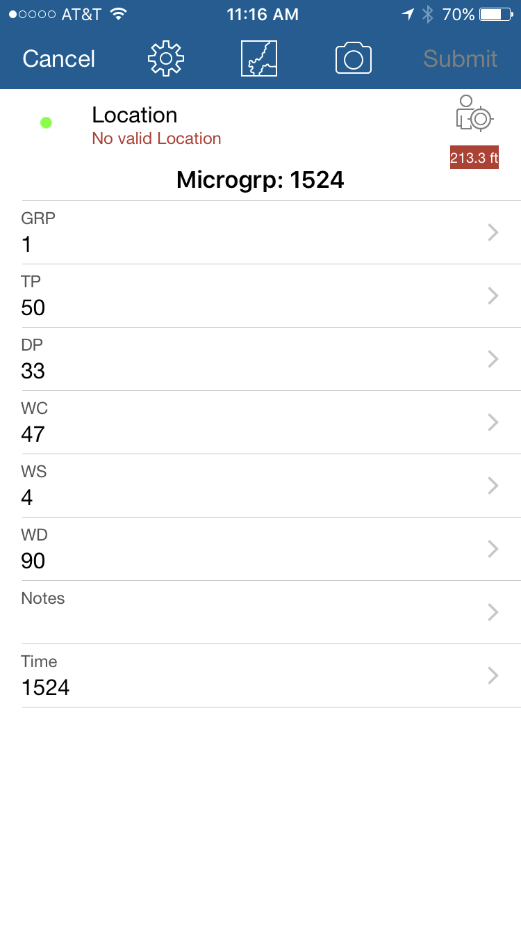
  Below, in figures 9.3 and 9.4 is what the map and attribute screen looked like in the Collector for ArcGIS app. The attribute information shown in figure 9.3 is for the point where the arrow is in figure 9.3. 

Fig 9.2: Map Used by the app

Fig 9.4: Attribute Information Screen on the app

Reorganizing Data After Data Collection

  After all of the data was collected for the 24 intersections, it was realized that the intended purpose of the study which was to see how road hierarchy, speed limit, and yellow light duration relate with each other, couldn't be solved with the way the attributes were organized. 

  The first issue with the attributes was that the road names and speed limits were not organized based on road hierarchy. They were organized randomly. These were reorganized by adding new fields names LongestLightTime, ShortestLightTime, HighestSpdLmt, LowestSpdLmt, and RelativeRdHierachy. This had to done because for each point collected, there were two yellow light times, two speed limits, and two road hierarchies. The road hierarchy was changed to more of a Boolean data type. Intersections were reclassified as having equal road hierarchies or not equal road hierarchies. Reclassifying the data into these new attributes fields would help to make creating maps and calculating other statistics easier. 

  Also, a mistake was made when originally creating the time field. The datatype was set to text, but in order to map it, the a new field was created with a short integer data type and the same values from the old time field were used.

  Going back to the study question to see how these attributes relate with each other, 4 calculated fields were created in ArcMap. The first one was the difference between the highest yellow light time and the lowest yellow light time by intersection. The second one was the difference between the speed limits of the two roads at the intersection. The third one was the shorter light time divided by the speed limit of the shorter yellow light. Lastly, the fourth one was the larger light time divided by the speed limit of the longer yellow light.

Results / Discussion

  This first map, shown below in figure 9.5, shows the location of the intersections studied. Most of the lights studied were in downtown, but 7 of them were located along Clairemont Ave. Almost all of the 4 way intersections within the study area were accounted for. 

Fig 9.5: Studied Intersections

  This next map, displayed in figure 9.6, shows the duration of the longer of the two yellow lights at each intersection. The map also has labels for each intersections which indicate whether or not the hierarchy at the road was equal or not.

  Based on this map, there is a relationship between road hierarchy and duration of yellow lights. Many of the roads located in the downtown part of the study area had the same hierarchy and had no difference between the yellow light times for both roads at the intersection. On the flip side, all of the intersections which are classified as having not equal road hierarchy are located along Clairemont Ave or Highway 37 and have a difference between the yellow light times between the two roads at the intersection. Interestingly, there was one intersection located on Water St. and 5th Ave which had an equal road hierarchy, but a difference in the yellow light length. However, this is the only case in which this happens. The map shows a that a difference in road hierarchy correlates with a difference in yellow light times.

Fig 9.6: Difference in Yellow light Times Between Roads by Intersection

  The next map, shown below in figure 9.7, shows the speed limit difference between the two roads at the intersection and compares it to the road hierarchy.
  This map looks fairly similar to the difference in yellow light length map. However, in this map, there were quite a few roads in downtown which had difference in speed limits of 5 mph. This because about half of the roads in downtown had a 25 mph speed limit, and the other half had a 30 mph speed limit.
  Every intersection which was classified as Not Equal except for one had a difference in speed limits of 15 mph. The speed limit of the faster roads (Clairemont Ave and Highway 37) were 45 mph and the speed limits of the slower roads were only 30 mph. There is one outlier within the traffic intersections. It is the traffic intersection of Clairemont Ave and Highway 37. The reason why there is a difference between hierarchies at this light where there is no difference between speed limits is because this is where Highway 37 ends which made for collecting attributes difficult to choose.
  Based off this map, a difference in road hierarchy at an intersection is almost certainly going to mean that there is a difference in speed limits between the roads. 

Fig 9.7: Difference in Speed Limits Between the Two Roads by Intersection

  Next, an interactive map was created in ArcGIS online to attempt to normalize the length of the longer yellow light by the speed limit of the corresponding road. The speed limits of the corresponding roads are labeled for reference and analysis. The values represented by the graduated circles are equal to the length of the longer yellow light at the intersection divided by the corresponding road speed limit. This gives a standardized value which makes the yellow light duration values comparable across intersections no matter the speed limit.
  This value can be seen as a time value for which a driver would have time to react. Interestingly, there is greater time for the driver to react when the speed limit is slower. This occurs in downtown mainly, but is really just where the speed limit is 30 mph or lower. A driver would have less time to react when traveling at higher speeds such as along. This occurs on Clairemont Ave and Highway 37 where the speed limit is 45 mph.
  This map points out that although the length of a yellow light generally increased with speed limit, it does not do so proportionally. Instead, the ratio between light length and speed limit decreases as the speed limit increases.

Interactive Ratio Map Between Yellow Light Duration and Speed Limit of the Higher Hierarchy Road

  A very similar kind of map was created in ArcMap, but with the lower hierarchy roads. This map, below in figure 9.8, shows the yellow light duration to speed limit ratio between the lower hierarchy roads at the intersections. Most of the trends shown in the previous map are presented in this map as well. However, there is one major difference. The difference is that there is a decreased yellow light time to speed limit ratio at the intersections located along Clairmont Ave and Highway 37 even though the speed limits are the same as they are in downtown.
  Perhaps this is because these are the intersections where the road hierarchy is not equal. These shortened ratios indicates that these lights for the lower hierarchy roads located along Clairmont Ave and Highway 37 have a shorter yellow light length than the lights near downtown and Water Street.

Fig 9.8: Lesser Hierarchy Yellow Light Time to Speed Limit Ratio

  This last map displayed below in figure 9.9 shows the time at which the data for each point was collected. The smaller the circle, the earlier that intersection was studied. The larger the circle, the later that intersection was studied. The route taken to collect the data can be seen by this map. The data collector started off in the southeast portion of the map and then collected data up though downtown, crossing the river on Madison street over to Clairmont. From there the data collector went back to collect data for two intersections along 5th Ave and then finished with the final four intersections located along Clairmont in the southern portion of the map.
  It is possible that the duration of yellow lights changes through out the day. There was one instance where the length of the yellow light changed while attempting to measure it several times. If this can happen at one intersection, it could certainly happen at others. For this reason, it was important that the data be collected quickly so that the variable of time didn't become a major contributing factor to the length of yellow lights.

Fig 9.9: Time at Which the Data Were Collected

Other Attribute Information
  The other attribute information such as notes and the street names was either used to help create the new fields to help explain the correlations, or didn't contain enough information where a map could be created.

Conclusion

  The results of this lab found many correlations between the attributes of road hierarchy, road speed limit, and length of yellow lights. It was discovered that when the road hierarchy of two roads at an intersection isn't equal, there is likely to be a difference in the length of the yellow light times. This also indicates that roads with a higher hierarchy have a longer yellow light and that roads with a lesser hierarchy have a shorter yellow light. It was also found that when the speed limit between two roads is different the difference between the yellow light duration is also different. Another important finding was that where the hierarchy of roads isn't equal, the ratio between yellow light time and speed limit was lower than when the hierarchy of roads was equal.
  If this project was to be done over again, a couple adjustments would be made when setting up the attributes. First, the road names would be organized by hierarchy where the road with the higher hierarchy would be always placed in Rd1Name and the road with the lower hierarchy would be placed in the Rd2Name. The second main change would be the road hierarchy classification. Instead of actually listing the road hierarchy, a relative hierarchy rank could be given. These values would be Greater, Equal or Lower.
  If one were to expand on this project. That person should should make the attribute changes listed above. They could also try to collect data on the age of the stoplight. Different aged stoplights are likely to have different yellow light times. Also, the study area could be larger, so that many more intersections could be looked at.

Arc Collector: Part 1, Gathering Weather Data

Introduction

  Collector for ArcGIS is a mobile app which allows for easy data collection while in the field. It allows for real time updates, domain restrictions for attributes, and photo attachment for specific locations. Multiple people can collect and submit data at the same time. This is very beneficial. If people need data be collected very quickly, the Collector for ArcGIS app is an extremely useful tool. Domains can be set up for the attributes which help to standardize the data and prevent data entry error. 

 For this lab, the Collector for ArcGIS app was used to collected attributes of weather data on Wednesday, March 29th between 3:30 pm and 5:00 pm. These attributes include group number, temperature, dew point, wind chill, wind direction, wind speed, time, and notes. The study area for this lab was all of UW-Eau Claire campus. Most of the study area was near campus buildings, but part of the study area was located down by the Chippewa river. The study area can be seen below in figure 8.0. The class was divided into 7 different groups each assigned to a zone to collect data on a specific part of campus. The different group zones can be seen in figure 8.1. Zones 4 and 5 are located on upper campus, zones 3,6 and 7 are located on lower campus on the south side of the river, and zones 1 and 2 are located on lower campus on the north side of the river. Each student was paired with another student to collect data within a zone. The author of the blog was assigned to group 1 which collected data for zone 1.

  

Fig 8.0: Study Area

Fig 8.1: Group Zones

Methods

Setting up the Collector for ArcGIS App

  Before collecting the weather attribute data and point data, the domains, ranges, and attribute names had to be set up. This was done when creating the feature class in the geodatabase for the project. 

Collecting the Point and Attribute Data

 Fig 8.2: Pocket Weather Meter

  A pocket weather meter and compass was used to collect the weather data. The weather pocket meter can be seen on the right in figure 8.2. Then, the weather data was entered into the Collector for ArcGIS app. While in the field, the map in the app had a nice basemap with a bunch of points which other people had collected. This can be seen below in figure 8.3 on the left. To add a point. the white plus button was tapped. The attribute data entry page was then opened. The attribute screen can be seen in figure 8.4 below on the right. GRP is the group number, TP is the temperature, DP is the dew point, WC is the wind chill, WS is the wind speed, WD  is the wind direction, Notes is the notes, and Time is the time. The units for TP, DP, and WC was °F, for WS it was mph, for WD it was degrees, and for Time it was military time with no colon. After entering in the attribute information, the Submit button was clicked to add the point and attribute information to the map.                    

                                                                                                                                                                  

  

Fig 8.3: Map for collecting data points

Fig 8.4: Attribute Screen 

Making Maps

  Next, a series of maps were created. The geodatabase was available to be copied from ArcGIS online because the map was shared with the class group which the class had access to. The maps for TP, WC, and DP were interpolated using the IDW method and the WS and WD attributes were used to create a wind vector map. No map was created for the Time or Notes field as the dat a wouldn't display very well in a map. One map was created on ArcGIS online displaying the temperatures.

Results / Discussion

  This first map, below in figure 8.5, shows the location of the data points collected by everyone. For each zone, there were two people collecting attributes, the collection points are distributed very randomly across campus. Each person was asked to collect 20 data points within their zone.

Fig 8.5: Data Collection Points

  This next map, below in figure 8.6, shows the temperature interpolated with the IDW method from the temperature values at each point. There are several areas of warm and cold spots throughout the map. Many of the differences are very slight as the range between the highest and lowest temperatures is only 12.9 °F, the average is 52.3 °F and the standard deviation is 2.4°F. The warm spots seem to more isolated than the cold spots are. This is probably because these values have some error associated with them. This is because the pocket weather meters were most likely not acclimated to the air temperature when students began taking their measurements. They were probably still cooling to the outside temperature as they just came from being inside.

Fig 8.6: Temperature Interpolation

  Next, an interactive map created in ArcGIS online is featured below. It is a proportional circle map. The larger the circle means the higher the temperature. The patterns in this map are the same as the map above as the same data is used, but is just displayed differently. The higher temperatures tend to be fairly isolated and probably occurred because people didn't wait for their pocket weather meter to get an accurate reading.

Interactive Temperature Map

  This next map, shown below in figure 8.7, displays the IDW interpolation of the WC values. This map is very similar to the temperature map. This is because the wind was very light when the data was collected for this lab and windchill is dependent on air temperature and wind. However, there is a bit more variation between the wind chill values than the temperature values. For the dew point values, the average was 51.8 °F, the standard deviation was 2.7 °F, and the range was 18 °F. The possible error for the windchill values is the same as the temperature values because wind chill is so dependent on air temperature.

Fig 8.7: Wind Chill Interpolation

  This next map, shown below in figure 8.8, shows the IDW dew point interpolation based on the data points. Similar to the temperature and wind chill maps, there appears to be isolated areas of high dew points. There is a sharp contrast in the dew points between upper and lower campus. The higher dew points seem to be located on lower campus, and the lower dew points seem to be located on upper campus and in zone 1. For the dew point values, the average was 39.1 °F, the standard deviation was 8.1 ­°F, and the range was 28 °F. The dew points seem to be isolated depending on the location in zones 2, 3, 6, and 7. In zones 1, 4, and 5, the dew points were very stable throughout. This is probably because there was some error in some of the values collected in zones 2, 3, 6, and 7. The reasons for this error is probably one of two reasons. One, people accidentally recorded the temperature value as the dew point value, or two, people didn't allow for their pocket weather meter to acclimate to the outside conditions before collecting data.

Fig 8.8: Dew Point Interpolation

  This next map, shown below in figure 8.9, displays the wind speed and direction. The arrows point in the direction of the wind flow, and the size of the arrow is based off of the wind speed. In zones 1,2 and 3, the wind direction is primarily from the east. In zones 4 and 5, the wind direction is mainly from the southeast. In zones 6 and 7 the wind direction seems to be random as there are wind directions from every direction. The wind speed seems to differ from zone to zone as well. Near buildings, the wind speed is generally lighter and in open areas such as in parking lots, fields, and on the bridge, the wind speed is generally greater. For the wind speed values, the average is 2.1 mph, the standard deviation is 2.5 mph, and the range is 33 mph. An example of possible error while collecting wind speed and direction data is that people didn't hold up the pocket weather meter long enough for the device to record a wind speed. Another example could be that people didn't know how to find the wind direction with the compass.

Fig 8.9: Wind Speed and Direction.

Other Attribute Information
  The Time, and Notes attributes were not standardized enough to make maps. The Time values were supposed to be entered as military time without a colon. Many people entered in the time values incorrectly and inserted a colon. This issue could be solved if the Time field was set to an integer data type, and a domain was created so only four numbers could be entered. The data type of the Notes attribute was accidentally set a numeric, so many people didn't enter in any notes. This could be fixed by making the data type text so that actual notes could be entered.

Conclusion

  This lab demonstrated the power of Collector for ArcGIS. Multiple people were able to easily collect and submit data which everyone could see in real time. The only issue with having so many people collect data is that people have slightly different ways of collecting it. For example, people held the pocket weather meter for varying amounts of time to record the wind speed. Collector for ArcGIS could be used for many different applications. It could be used to collect information about utilities, such as the condition of telephone poles. Collector for ArcGIS also allows for everyone to see where the people collecting data are at. This could be useful in a work setting so that a supervisor could see where the employee is collecting data at to make sure they are staying on task. The goals of collecting the weather attribute information were met. 240 points were collected with only about 14 people in just a little over an hour and a half. Much of this data was standardized and was very easy to create into a maps.