Arc Collector: Part 1, Gathering Weather Data

Introduction

  Collector for ArcGIS is a mobile app which allows for easy data collection while in the field. It allows for real time updates, domain restrictions for attributes, and photo attachment for specific locations. Multiple people can collect and submit data at the same time. This is very beneficial. If people need data be collected very quickly, the Collector for ArcGIS app is an extremely useful tool. Domains can be set up for the attributes which help to standardize the data and prevent data entry error. 

 For this lab, the Collector for ArcGIS app was used to collected attributes of weather data on Wednesday, March 29th between 3:30 pm and 5:00 pm. These attributes include group number, temperature, dew point, wind chill, wind direction, wind speed, time, and notes. The study area for this lab was all of UW-Eau Claire campus. Most of the study area was near campus buildings, but part of the study area was located down by the Chippewa river. The study area can be seen below in figure 8.0. The class was divided into 7 different groups each assigned to a zone to collect data on a specific part of campus. The different group zones can be seen in figure 8.1. Zones 4 and 5 are located on upper campus, zones 3,6 and 7 are located on lower campus on the south side of the river, and zones 1 and 2 are located on lower campus on the north side of the river. Each student was paired with another student to collect data within a zone. The author of the blog was assigned to group 1 which collected data for zone 1.

  

Fig 8.0: Study Area

Fig 8.1: Group Zones

Methods

Setting up the Collector for ArcGIS App

  Before collecting the weather attribute data and point data, the domains, ranges, and attribute names had to be set up. This was done when creating the feature class in the geodatabase for the project. 

Collecting the Point and Attribute Data

 Fig 8.2: Pocket Weather Meter

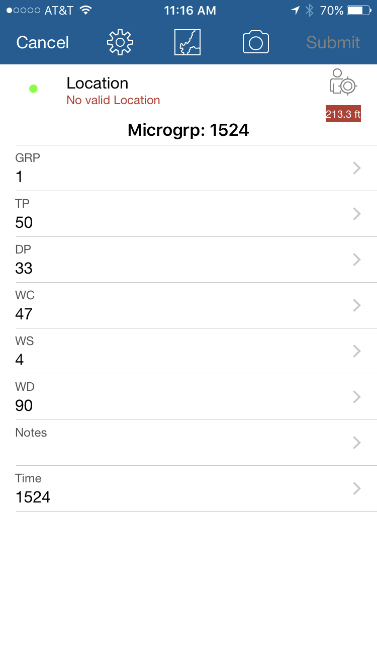
  A pocket weather meter and compass was used to collect the weather data. The weather pocket meter can be seen on the right in figure 8.2. Then, the weather data was entered into the Collector for ArcGIS app. While in the field, the map in the app had a nice basemap with a bunch of points which other people had collected. This can be seen below in figure 8.3 on the left. To add a point. the white plus button was tapped. The attribute data entry page was then opened. The attribute screen can be seen in figure 8.4 below on the right. GRP is the group number, TP is the temperature, DP is the dew point, WC is the wind chill, WS is the wind speed, WD  is the wind direction, Notes is the notes, and Time is the time. The units for TP, DP, and WC was °F, for WS it was mph, for WD it was degrees, and for Time it was military time with no colon. After entering in the attribute information, the Submit button was clicked to add the point and attribute information to the map.                    

                                                                                                                                                                  

  

Fig 8.3: Map for collecting data points

Fig 8.4: Attribute Screen 

Making Maps

  Next, a series of maps were created. The geodatabase was available to be copied from ArcGIS online because the map was shared with the class group which the class had access to. The maps for TP, WC, and DP were interpolated using the IDW method and the WS and WD attributes were used to create a wind vector map. No map was created for the Time or Notes field as the dat a wouldn't display very well in a map. One map was created on ArcGIS online displaying the temperatures.

Results / Discussion

  This first map, below in figure 8.5, shows the location of the data points collected by everyone. For each zone, there were two people collecting attributes, the collection points are distributed very randomly across campus. Each person was asked to collect 20 data points within their zone.

Fig 8.5: Data Collection Points

  This next map, below in figure 8.6, shows the temperature interpolated with the IDW method from the temperature values at each point. There are several areas of warm and cold spots throughout the map. Many of the differences are very slight as the range between the highest and lowest temperatures is only 12.9 °F, the average is 52.3 °F and the standard deviation is 2.4°F. The warm spots seem to more isolated than the cold spots are. This is probably because these values have some error associated with them. This is because the pocket weather meters were most likely not acclimated to the air temperature when students began taking their measurements. They were probably still cooling to the outside temperature as they just came from being inside.

Fig 8.6: Temperature Interpolation

  Next, an interactive map created in ArcGIS online is featured below. It is a proportional circle map. The larger the circle means the higher the temperature. The patterns in this map are the same as the map above as the same data is used, but is just displayed differently. The higher temperatures tend to be fairly isolated and probably occurred because people didn't wait for their pocket weather meter to get an accurate reading.

Interactive Temperature Map

  This next map, shown below in figure 8.7, displays the IDW interpolation of the WC values. This map is very similar to the temperature map. This is because the wind was very light when the data was collected for this lab and windchill is dependent on air temperature and wind. However, there is a bit more variation between the wind chill values than the temperature values. For the dew point values, the average was 51.8 °F, the standard deviation was 2.7 °F, and the range was 18 °F. The possible error for the windchill values is the same as the temperature values because wind chill is so dependent on air temperature.

Fig 8.7: Wind Chill Interpolation

  This next map, shown below in figure 8.8, shows the IDW dew point interpolation based on the data points. Similar to the temperature and wind chill maps, there appears to be isolated areas of high dew points. There is a sharp contrast in the dew points between upper and lower campus. The higher dew points seem to be located on lower campus, and the lower dew points seem to be located on upper campus and in zone 1. For the dew point values, the average was 39.1 °F, the standard deviation was 8.1 ­°F, and the range was 28 °F. The dew points seem to be isolated depending on the location in zones 2, 3, 6, and 7. In zones 1, 4, and 5, the dew points were very stable throughout. This is probably because there was some error in some of the values collected in zones 2, 3, 6, and 7. The reasons for this error is probably one of two reasons. One, people accidentally recorded the temperature value as the dew point value, or two, people didn't allow for their pocket weather meter to acclimate to the outside conditions before collecting data.

Fig 8.8: Dew Point Interpolation

  This next map, shown below in figure 8.9, displays the wind speed and direction. The arrows point in the direction of the wind flow, and the size of the arrow is based off of the wind speed. In zones 1,2 and 3, the wind direction is primarily from the east. In zones 4 and 5, the wind direction is mainly from the southeast. In zones 6 and 7 the wind direction seems to be random as there are wind directions from every direction. The wind speed seems to differ from zone to zone as well. Near buildings, the wind speed is generally lighter and in open areas such as in parking lots, fields, and on the bridge, the wind speed is generally greater. For the wind speed values, the average is 2.1 mph, the standard deviation is 2.5 mph, and the range is 33 mph. An example of possible error while collecting wind speed and direction data is that people didn't hold up the pocket weather meter long enough for the device to record a wind speed. Another example could be that people didn't know how to find the wind direction with the compass.

Fig 8.9: Wind Speed and Direction.

Other Attribute Information
  The Time, and Notes attributes were not standardized enough to make maps. The Time values were supposed to be entered as military time without a colon. Many people entered in the time values incorrectly and inserted a colon. This issue could be solved if the Time field was set to an integer data type, and a domain was created so only four numbers could be entered. The data type of the Notes attribute was accidentally set a numeric, so many people didn't enter in any notes. This could be fixed by making the data type text so that actual notes could be entered.

Conclusion

  This lab demonstrated the power of Collector for ArcGIS. Multiple people were able to easily collect and submit data which everyone could see in real time. The only issue with having so many people collect data is that people have slightly different ways of collecting it. For example, people held the pocket weather meter for varying amounts of time to record the wind speed. Collector for ArcGIS could be used for many different applications. It could be used to collect information about utilities, such as the condition of telephone poles. Collector for ArcGIS also allows for everyone to see where the people collecting data are at. This could be useful in a work setting so that a supervisor could see where the employee is collecting data at to make sure they are staying on task. The goals of collecting the weather attribute information were met. 240 points were collected with only about 14 people in just a little over an hour and a half. Much of this data was standardized and was very easy to create into a maps.